Jekyll2025-08-14T15:02:11+00:00https://diffuse.science/feed.xmlThe Diffuse ProjectThe Diffuse ProjectFrom systems operators to systems architects2025-08-13T00:00:00+00:002025-08-13T00:00:00+00:00https://diffuse.science/diffuse-blog-postWhat if the next PDB is… the PDB?
We just launched The Diffuse Initiative, a new project to experimentally study protein motion and rethink how we generate scalable, useful X-ray data for the scientific community.
]]>Seemay ChouEncoding data for a protein dynamics centered AlphaFold2025-08-12T00:00:00+00:002025-08-12T00:00:00+00:00https://diffuse.science/posts/encodingThe breakthroughs of AlphaFold and its successors galvanized both biology and machine learning communities. What enabled this revolution? High-quality, standardized data openly organized for all to use.
For decades, structural biology has relied on the Protein Data Bank (PDB), a remarkable archive of macromolecular structures. Its standardization made large-scale machine learning possible, creating the conditions that allowed AlphaFold to thrive. But while AlphaFold changed our expectations for static structure prediction, the next frontier is dynamics, and here, our data infrastructure is still stuck in the past.
Exciting, much of this information on dynamics is already encoded in the raw experimental data we’ve been collecting for decades, and more information is being gleaned from expanding data collection in diffuse scattering. Yet our current data formats are built for single, static models, making them ill-suited to capture loop motions, alternate side-chain conformations, ligand-induced flexibility, or compositional variation.
As a result, much of this rich information is lost, limiting both the biological insights we can draw and the conclusions AI algorithms can reach. We are working to change that. If AlphaFold’s success was fueled by standardized, static structures, imagine the possibilities if we could deliver standardized, machine-readable, and human-interpretable representations of dynamic structures.
As we have written about before, we envision a hierarchical, ensemble-aware encoding framework designed to capture the full complexity of macromolecular dynamics. This includes distinguishing between different sources of heterogeneity, such as conformational changes versus compositional variation, and representing them in a nested structure that reflects the true physical states. Beyond encoding a single model, this would enable searches based on dynamic properties—for example, identifying all proteins where a particular loop adopts multiple conformations or where ligand binding alters flexibility in a neighboring site. To enable AI co-driven discovery, these representations must serve both human reasoning and machine learning, which means encoding at the individual model level and making this data practical for researchers to access, adapt, and integrate into their pipelines. Such a system would not only help scientists interpret complex structures but also establish community benchmarks, uncover systematic errors, and accelerate method development.
Our goal is to re-engineer the encoding and infrastructure of structural biology to embrace dynamics and set the stage for the next revolution, one where machine learning models not only predict what a protein looks like but also how it moves and functions.
]]>Stephanie Wankowiczstephanie@wankowiczlab.comModeling Protein Dynamics2025-08-12T00:00:00+00:002025-08-12T00:00:00+00:00https://diffuse.science/posts/modelingThe Diffuse Project is developing new methods for collecting and modeling protein dynamics. One of the most exciting aspects of this emerging frontier is that the details of these ensembles are often already hidden in plain sight, embedded within the experimental data used to generate the static structures. We hypothesize that if we can learn directly from this raw experimental data, we may be able to more accurately reconstruct a macromolecule’s conformational ensemble.
At present, we often model ensembles separately from Bragg peaks, the sharp, well-defined signals from crystallography, and diffuse scattering, the information-rich “background” patterns. The results rarely match. We aim to change that by transitioning to a paradigm where we directly learn from experimental data, integrating both Bragg and diffuse scattering to create consistent, physically grounded models of a macromolecule’s ensemble.
Our approach begins by improving how experimental data is integrated into modeling, building tools that incorporate both Bragg and diffuse data into optimization and machine learning loss functions and validation metrics, and improving algorithms for ensemble modeling directly from Bragg data. We are also moving towards developing machine learning algorithms that train directly on experimental data rather than using it only in the loss function.
Ultimately, we envision a representation learning framework that dissolves the boundaries between experimental modalities, bringing Bragg, diffuse, and other structural data types into a single, shared space. Within this unified representation, molecular dynamics simulations informed by diffuse data will flow seamlessly into Bragg-based training and inference, allowing the strengths of each approach to amplify the other. By enabling AI models to learn jointly from heterogeneous datasets, we can unlock new levels of predictive accuracy, reveal hidden relationships between data types, and open the door to true cross-modality discovery in structural biology.
]]>Stephanie Wankowiczstephanie@wankowiczlab.comJoin diffUSE!2025-08-05T00:00:00+00:002025-08-05T00:00:00+00:00https://diffuse.science/posts/jobsWe currently have three positions open on the diffUSE team through Astera.
1) Machine Learning Scientist
Description:
The Diffuse Project is seeking a Machine Learning Scientist to join a multidisciplinary team developing machine learning methods to extract hidden functional states from experimental structural biology data (i.e. electron density, structure factors, diffraction patterns, etc.). We are particularly interested in applicants with deep expertise in generative modeling, reinforcement learning, or representation learning who are excited to apply these approaches to real-world structural data. We aim to develop a new generation of tools that treat experimental data as central inputs to model training, validation, and discovery. This role is part of a highly interdisciplinary team of machine learning experts, structural biologists, and biophysicists. Apply here
2) Machine Learning Infrastructure Engineer
Description: The Diffuse Project is seeking a Machine Learning Infrastructure Engineer to lead the development of robust, scalable backend systems that power machine learning–driven discoveries in structural biology. You will work at the intersection of scientific research and software engineering, working with researchers to train, test, and deploy ML models directly on experimental data (electron density/structure factors) coming from X-ray crystallography and cryo-EM. This role is ideal for someone with deep experience in ML infrastructure and scientific computing who thrives in a collaborative and product-minded environment. This is a 6-month assignment with potential for extension. Apply here
3) Software Engineer
Description: The Diffuse Project is seeking a Software Engineer to join a multidisciplinary team working to expand the frontier of structural biology by developing methods to capture protein motion. We are assembling a team to develop the process for collecting and interpreting this data from data collection to the final interpretation and scientific impact. You will develop open-source software products to process experimental structural biology data and to manipulate protein structural models. We are particularly interested in product minded applicants who have worked to build products for scientists or other disciplines where a close interface with your users was critical. Apply here
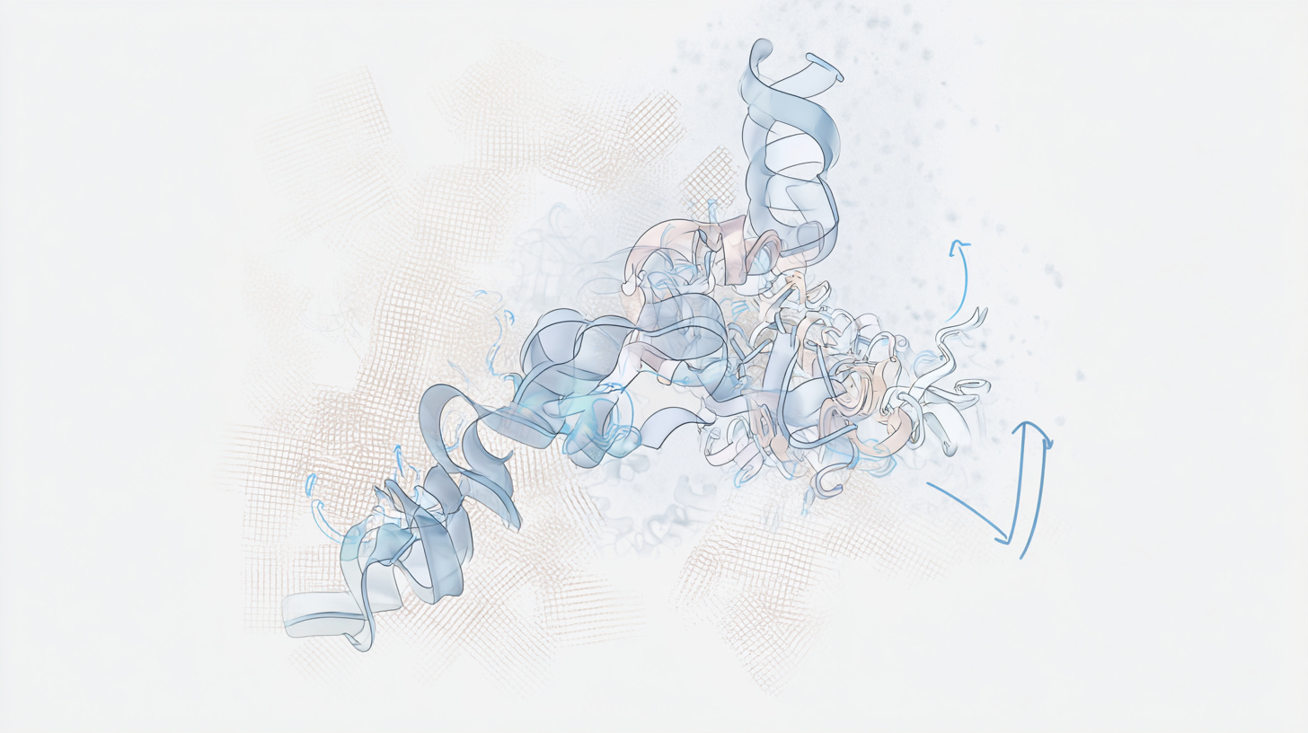
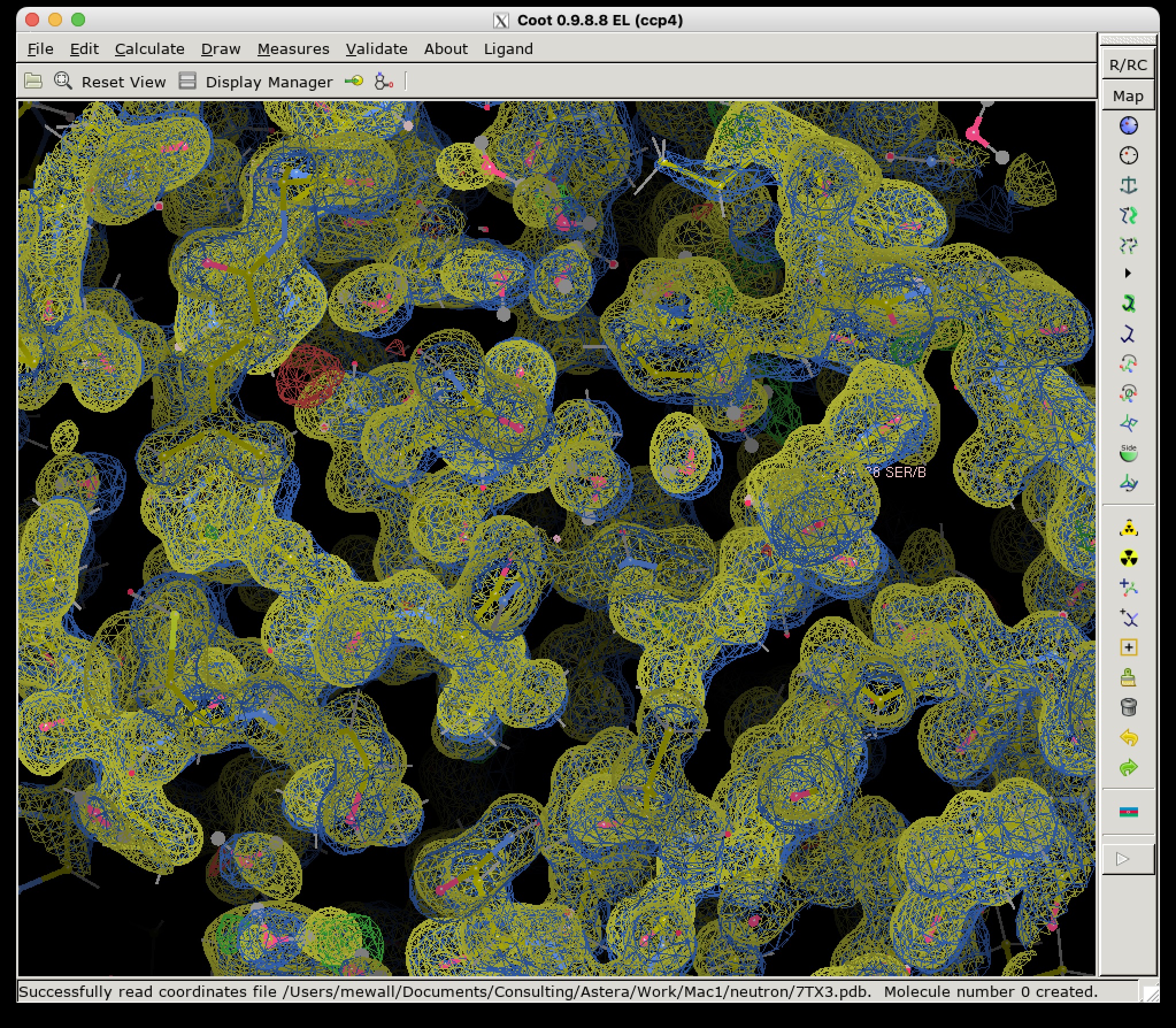
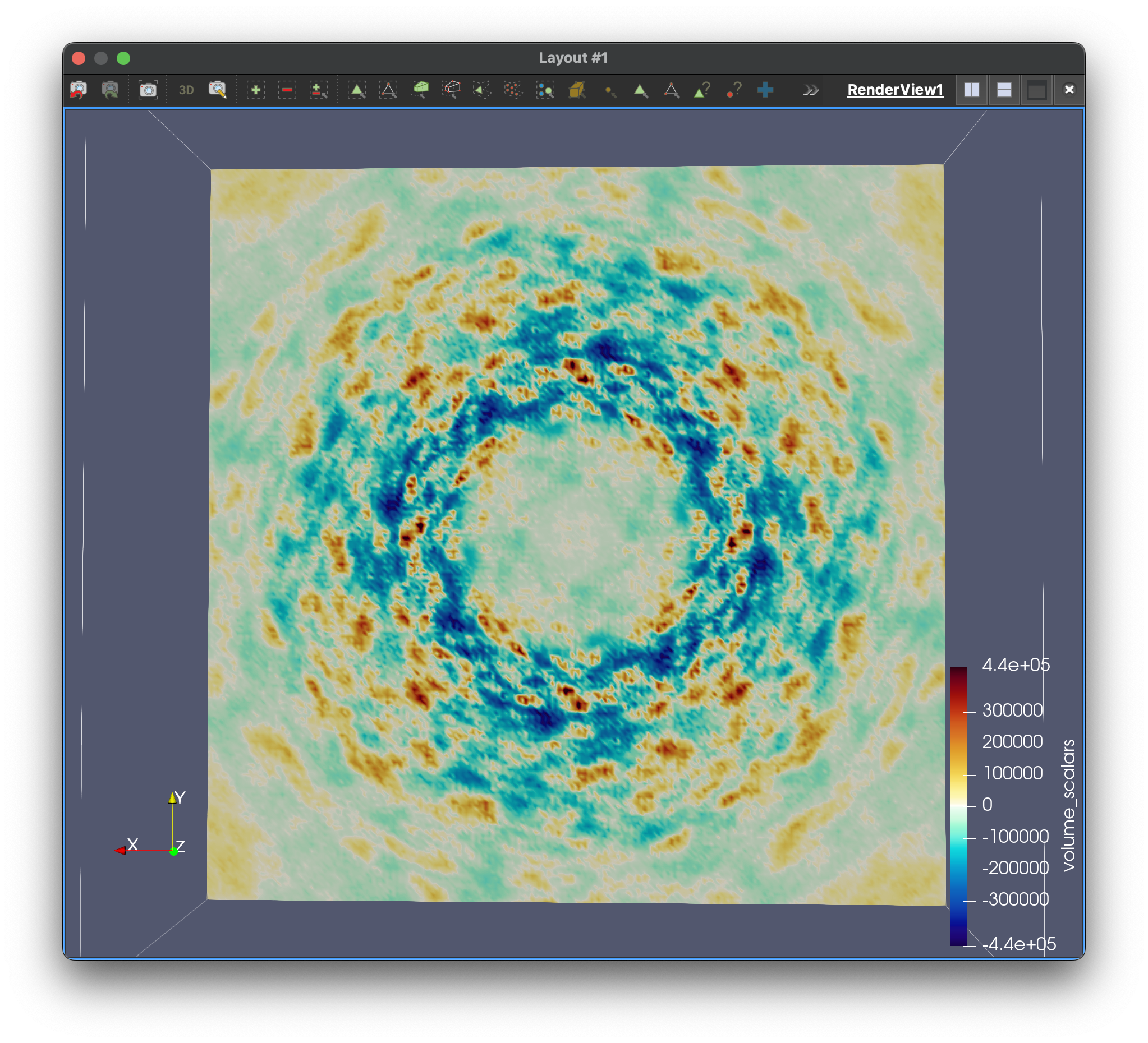
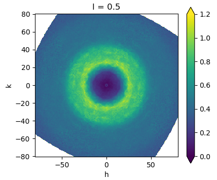
]]>Stephanie Wankowiczstephanie@wankowiczlab.comLet’s dance!2025-08-05T00:00:00+00:002025-08-05T00:00:00+00:00https://diffuse.science/post/lets-danceFirst diffUSE MD simulations of diffraction. (Left) Visualization of the MD trajectory. (Center) Electron density from simulated Bragg data at 1-sigma (yellow) overlaid with experimental 2FoFc (blue). (Right) Slice through the computed diffuse scattering map.
We want to know all about how proteins “dance” in the crystal. In addition to having their own individual moves (see the DaVinci Dude Dance post), different proteins can’t occupy the same space at the same time, and sense and respond to their neighbors, even at a distance.
Molecular-dynamics simulations give us a picture of the whole choreography. Starting with the crystal structure, our simulations evolve using assumptions about the underlying physics. The motions appear random but follow patterns that show up in the diffraction. Right now researchers can make molecular-dynamics simulations agree reasonably well with the diffraction data, but the agreement isn’t perfect. In particular, so far the simulations haven’t done a very good job of modeling both the Bragg and diffuse data simultaneously.
We’re working to fix this problem.
Our first simulations are especially important, as they’ll serve as a reference to assess our progress. Inspired by the project’s first experiments during the diffUSE kickoff meeting (see Getting our feet wet post), we’re performing simulations of SARS-Cov-2 Nsp3 macrodomain, the subject of a beautiful neutron crystallography study done in the Fraser lab.
Above is a first look at the initial results. In the movie, the waters look like swarming gnats, the ions are balls, and the proteins are cartoon ribbons. The proteins wave around and also jostle their neighbors. Waters and ions diffuse and sometimes stick to the protein for a while.
The simulated electron density in the center panel shows the average picture. It doesn’t give us information about how atoms move together, but diffuse scattering does (right panel). Combining both will enable us to develop more accurate MD models of protein crystals.
Methods
The lunus repository has some examples of how to prepare crystalline MD simulations and use them to analyze Bragg and diffuse data.
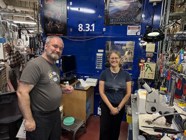
]]>Michael Wallmewall00@gmail.comGetting our feet wet2025-07-30T00:00:00+00:002025-07-30T00:00:00+00:00https://diffuse.science/posts/wetfeetTeam diffUSE convened at Astera HQ in Emeryville, CA on June 23-24, 2025. The whole visit was a treat – meeting brilliant people, brainstorming new ideas – but for me, the highlight was an impromptu trip up the bay for a wee bit of X-ray data collection.
Getting our feet wet at ALS 8.3.1
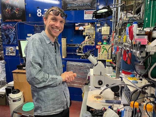
ALS beamline 8.3.1 is hallowed ground. Although I’ve seen it before on previous trips, this was my first time collecting data there. What fun!
We were aided in our quest by Galen Correy (Fraser Lab at UCSF) who donated a tray full of beautiful SARS-CoV-2 Nsp3 Macrodomain crystals. Galen and collaborators have done some amazing crystallography with this system: check out their ligand-screening campaign and neutron diffraction experiments. As we discovered at ALS that afternoon, it also has beautiful diffuse scattering!
This is a calculated diffraction pattern in false-color intensity (red is bright, black is dark). Upper insets represent two different dance moves, both of which could be represented by the Vitruvian Man, but the coordinated motions are lost if all you have is the time-averaged image in black-and-white (middle inset). Bottom insets are backbone traces of the actual protein molecules used to calculate the diffraction. The tiny little specks peppering the image are the Bragg spots, which define the average appearance of the molecule over time. Almost everything we know about atoms comes from Bragg data. All that stuff in between the Bragg spots is the Diffuse Scatter, and it tells us how the atoms dance.
The pattern on the left side corresponds to a particular 2-state molecular motion that is too subtle to see without zooming in. The pattern on the right has all the atoms in the same positions, but at different times. Regions colored in red have the opposite direction that they do on the left. Just like your arms do if you are doing jumping jacks vs doing “The Wave”.
The two diffuse patterns are similar, but clearly different. A major goal of the diffUSE project is to get the weak signal of diffuse scatter measured clearly enough to be analyzed unambiguously in this way.
Script for converting a two-conformer pdb file into diffuse scatter data.
]]>James Holtonjmholton@lbl.govEmbrace the Mess2025-07-29T00:00:00+00:002025-07-29T00:00:00+00:00https://diffuse.science/posts/ligandsThree new papers from Roche, accompanied by a perspective by Elspeth Garman, describe a fantastic ligand–protein structural dataset. They focus on several related fatty acid-binding proteins (FABPs) and report 229 high-resolution ligand-bound structures. The first paper explores how protein dynamics (and allosteric interactions with membrane mimics) change when empty lipid-binding sites are filled by natural or synthetic ligands. The second examines detailed atomistic interactions across isoforms, with lessons for selectivity. Along the way, there is great crystallographic lore: nearly isomorphous crystals, twinning, and more. The third paper focuses on how ligand chemistry can often be mis-assigned due to complexities in synthesis, isomerization, or transformation within the crystal. This is a problem we have observed ourselves in our macrodomain ligands and I expect to see more often as “make on demand” chemistry democratizes ligand soaking.
The authors distill these findings into a set of very conservative lessons: prioritize chemical certainty, gate on full occupancy, and filter out ambiguous cases before using structural data for machine learning. Elspeth echos some of these concerns in the perspective. I disagree. I think we need to consider these lessons differently depending on the use case:
Downstream medicinal chemistry or mechanistic interpretation without a structural biologist in the loop: If someone is simply taking the PDB as “truth” to guide synthesis, then rigorous filtering to avoid incorrect ligand identities is absolutely appropriate. I don’t think this actually happens anywhere, but this is always the straw man that such papers “warning” about the pollution of the PDB are concerned about. This includes papers criticizing our work (see also our response).
Medicinal chemistry fully integrated with structural biology: Here, strict filtering risks losing huge opportunities. Alternate conformations in both ligand and binding site, unusual B-factors, and subtle occupancy differences are not nuisances. These are the very signals that can inspire new design strategies and suggest unexplored mechanisms of selectivity.
Input to machine learning to predict protein ligand complexes: Curating only “gold-standard” data is going to be incredibly limiting. Disagreements between models and experimental data are opportunities to improve algorithms and better understand real-world uncertainty. I doubt that many of the structures that will be deposited by the OpenBind consortium will pass these filters.
Real experimental data is messy, full of alternate conformations, unexpected chemistries, and crystallization “oddities”. Filtering exclusively for perfection may feel safe, but it also limits discovery. Even though using coordinates of the partial occupancy ligands and static alternative conformations will improve things, I’m hoping that the ML for structural biology field will increasingly embrace the mess of experimental data more directly. I’ve written about this before from conceptual, practical, and policy perspectives. While this trio of papers represents a tremendous teaching text that guides the reader through many of the complexities of protein-ligand data sets, I disagree with the jeremiads at the end of these papers about the potential for misuse. I truly wish there were more careful papers like this out there.
]]>James Fraserjfraser@fraserlab.comNew website2025-07-22T00:00:00+00:002025-07-22T00:00:00+00:00https://diffuse.science/posts/new-websiteOur new website is hosted by Github Pages, and its source code can be viewed here.
]]>Daniel Hogandaniel.hogan@ucsf.edu