Coffee is for Closers: making Mac1 diffuse scattering reproducible

Anyone who has published a paper (or in our case, a Stack) knows the last 10% is the hardest part. Steve, Nozomi, Jaime, and I have been working on the core result for a while: apo Mac1 diffuse scattering that looks the same whether we collect it at CHESS in New York or ALS in California. What we’ve spent recent months on is moving from qualitative agreement “looks the same” to quantitative agreement “is the same, and here’s why.” Consider this a preview of the scholarly work to come.

Most of that effort was unglamorous: making the analysis reproducible, wrapping it in a pipeline, getting it to run the same way across different (and cloud) compute environments, etc. This is the hard part of open science. But doing it forced us to pin down every choice that feeds into a diffuse map, and in the process it deepened our understanding of what the result actually is and how firmly we can stand behind it.

Going into the project, we knew qualitatively that high-quality diffuse data depends on keeping the sample humid, avoiding radiation damage, and using large crystals. Now, we can show that when all three are in place, the maps agree across sites. Our best metric for this is the pairwise correlation coefficient between datasets, compared against a ceiling, or maximum expected correlation, set by the product of each dataset’s CC* (an estimate from its internal consistency (CC½) of how well it tracks the true underlying signal). This lets us ask how similar two datasets are given the noise in each. Across four beamtimes, two at CHESS, two at ALS, every pairwise CC sits at or near its ceiling, meaning the datasets are as similar as their noise allows, with no signature of which site collected them.

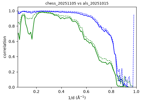
Figure legend: Correlation between a CHESS dataset and ALS dataset for the halo (blue) and non-halo (green) relative to the maximum expected correlation (dashed line).

And when one or more of the ingredients is systematically missing (whether on purpose or by accident), the maps clearly diverge, and we can trace the difference back to the piece that was left out. Our focus on reproducibility became the instrument for understanding our physical and computational workflows, setting the stage to help democratize diffuse scattering across more beamlines and users.

In addition to the headline result (diffuse scattering reproducible, yay!), this process gathered a pile of smaller lessons, mdx2 quirks and settings, and beamline configuration changes that we will describe fully in the Stack. Collectively, these lessons allowed us to strengthen our computational methods by identifying and fixing ‘one-offs’ such as a single hot pixel at the detector at CHESS ruining our ability to get quantitative agreement between sites. Without a standard mdx2 workflow, background subtraction can masquerade as signal, or we can accidentally misindex samples.

We are excited to have crossed the threshold of “reproducible diffuse scattering” and the full stack will enable others to join the party. This entire exercise shows that a major value of open science is raising our game to finish the work.